
How many different kinds of NBA players are there?
Introduction: NBA players
Recently, The Ringer grouped NBA players by how much they were worth seeing live and by how much they were worth in a trade to other NBA teams. In this post, I group NBA players by their performance using a clustering algorithm to understand the archetypes that played in the NBA last year.
The Python code I wrote to pull, scrub, and analyze the data is available on Github as a Jupyter notebook
In my analysis, I use three player stats (Points Per Game, Total Rebounds Per Game, and Assists per Game) to cluster players. I used stats from the 2017-2018 season. Data from a different year could yield different clusters since both the dynamics of the game and the roles individual players play on their team changes over time.
Results: How many different kinds of NBA players are there?
With per game data on 469 NBA players from the 2017-2018 season, I cluster the players and investigate the number and kind of archetypes that played in the NBA last year. The Python code I wrote to pull, scrub, and analyze the data is available on Github as a Jupyter notebook
Here’s what Points Per Game (PS/G), Total Rebounds Per Game (TRB), and Assists per Game (AST) look like for the 2017-2018 NBA season:
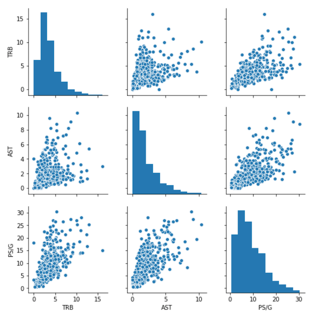
Above is a scatter plot matrix of PS/G, TRB, and AST for 469 players for the 2017-2018 NBA season. Note that each stat is on a different scale. I cluster the players using K-Means. To learn more about K-Means, see here. Since each stat is on a different scale, I center and scale each statistic by removing the mean value and dividing by the standard deviation before running K-Means.
After applying K-Means to the centered and scaled data, we found three clusters. For details on how I selected the number of clusters, see the Methods section below. Players were clustered according to the role they tended to play on their team for the 2017-2018 season resulting in three archetypes which we call Playmakers, Shot takers, and Role players:
Group A: Playmakers
- Representative players: LeBron James, Ben Simmons, J.J. Redick
- Group A average stats: 17.27 PS/G - 4.54 TRB - 5.31 AST
Group B: Shot takers
- Representative players: Klay Thompson, Robert Covington, Kelly Olynyk
- Group B average stats: 12.71 PS/G - 5.92 TRB - 1.90 AST
Group C: Role players
- Representative players: J.R. Smith, Danny Green, Andre Iguodala
- Group C average stats: 5.23 PS/G - 2.24 TRB - 1.23 AST
Methods: Notes on using K-Means and Python to perform this analysis
Selecting the number of clusters using model inertia and silhouette coefficients
Since we have to specify the number of groups to cluster the data into (K) before applying K-Means and we don’t know K a priori, we use the model inertia (total within-cluster sum-of-squares) and silhouette coefficient to determine K. To learn more about determining the number of clusters (K) in a data set, see here. Here’s what the inertia and silhouette look like for K = 1 to K = 10 clusters. Note that the silhouette isn’t defined for K = 1 cluster.
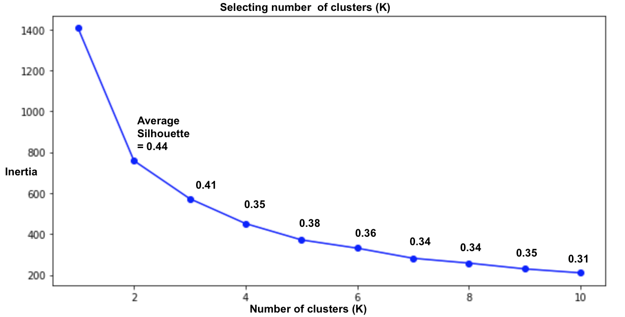
Above is a plot of Inertia vs Number of clusters (K) and each point is labeled with the average silhouette coefficient for K clusters. The inertia decreases as the number of clusters increases. We use it to determine the number of clusters by looking for the point K where there is an elbow in the plot. The silhouette coefficient for a sample ranges from [-1,1]. A value of +1 indicates the sample is far away from neighboring clusters and a negative value indicates the sample might be assigned to the wrong cluster. To learn more about the silhouette coefficient, see here.
Since the average silhouette coefficient at K = 2 and K = 3 are close and there isn’t an unambiguous elbow at those points, I chose to explore and run K-Means with K = 3 clusters.
Helpful resources
I found these resources helpful for getting started with and using Python to perform this analysis: